Tools/Suggestions

This page provides a collection of useful tools, scripts, and suggestions for CMS analysis workflows. Here you can find guidance for data handling, command-line utilities, and example scripts to streamline common tasks in a CMSSW or UNIX environment.

CMS UNIX (lxplus) tools

Finding files/Datasets using DAS CLI

The CMS DAS CLI lets users quickly find datasets and files within the CMS computing system. It works on any lxplus session with a valid VOMS proxy. Instructions can be found in the CMS DAS web-page.

• Simple DAS query that displays all the available datasets using wildcards:

dasgoclient --query="dataset=/Muon*/Run2023*-22Sep2023_v*/NANOAOD" | sort -V
              

• List all files in the dataset:

  
  dasgoclient --query="file dataset=/Muon0/Run2023C-22Sep2023_v1-v1/NANOAOD"
        

  It lists all the individual files in the dataset, with each file path on a separate line.

• Count the number of files:

  
  dasgoclient --query="file dataset=/Muon0/Run2023C-22Sep2023_v1-v1/NANOAOD" | wc -l
        

  It counts how many files are in the dataset, and outputs a single integer representing the number of files.

• Get dataset summary:

  
  dasgoclient --query="summary dataset=/Muon0/Run2023C-22Sep2023_v1-v1/NANOAOD"
        

  It provides metadata like number of events, total size, and creation date, in key-value format.

Directly downloading files using xrdcp

Find the tutorial for the XRootD dilesystem here. Downloading one file is easy. Find the full path of the file using DAS CLI commands and run xrdcp as follows.

xrdcp root://cmsxrootd.fnal.gov//store/data/Run2023C/Muon0/NANOAOD/22Sep2023_v1-v1/2530000/030eead5-93f9-405c-863c-a62244712e91.root .
            

I find it helpful to define the following function in my ~/.bashrc file.

get_from_das() {
  [ -z "$1" ] && echo "Usage: get_from_das <filename> [outputname]" && return 1
  cmd="xrdcp root://cmsxrootd.fnal.gov/$1 ${2:-.}"
  echo -e "\033[93mCommand:\033[0m \033[3;33m$cmd\033[0m"
  eval "$cmd"
}
            

Usage:

get_from_das /store/data/Run2023C/Muon0/NANOAOD/22Sep2023_v1-v1/2530000/030eead5-93f9-405c-863c-a62244712e91.root

Here I am using the redirector cmsxrootd.fnal.gov (server that acts as a middleman between client and the actual storage site) which is based in Fermilab. The following alternative redirectors are also available.

• cmsxrootd-global.cern.ch (global CMS XRootD redirector at CERN)
• xrootd-cms.infn.it (INFN, Italy)

For downloading files in bulk, I use the following two tools.

1. makelist.py : It runs DAS CLI to extract list of filtered files for the datasets mentioned in the script. It writes the output to a text file. CMS VOMS proxy is needed for this step. The usage is as follows:

   
   voms-proxy-init -voms cms
   python3 makelist.py -n 10 -min 100 -max 200 ## picks the first 10 files with sizes between 100 MB to 200 MB
                   

2. xrdcp_files.py : It runs xrdcp to download files listed in the text file.

   python3 xrdcp_files.py

Luminosity calculation using run-number and luminosity-section (JSON)

The brilcalc tool is available in lxplus at ~/.local/bin/brilcalc. It takes a JSON file as input, which contains run-number and lumisections in the following format.

{
  "321975": [[591, 593], [597, 599], [717, 734] , [736]],
  ....
}
            

This tool is run as follows.

brilcalc lumi \
  --normtag /cvmfs/cms-bril.cern.ch/cms-lumi-pog/Normtags/normtag_PHYSICS.json \  # Path to the normtag JSON with luminosity calibration constants
  -c web \                                                                        # Use web API as input source (avoids old Oracle DB issues)
  -u /fb \                                                                        # Output integrated luminosity in femtobarns (/fb)
  -i [[json file name]]                                                           # Input golden JSON file with certified lumisections
            

While running brilcalc, it is recommended (by LUM POG) to use a physics approved normtag (in this case, normtag_PHYSICS.json). This normtag json converts the numbers into physical units. More information can be found in the LUM POG TWiki page. The Golden JSONs corresponding to the Run-2 and Run-3 data taking periods can be found here.

Cross-section calculation using GenXSecAnalyzer

The GenXSecAnalyzer is used to calculate or extract the cross-section of a simulated process from the LHE level. I made a wrapper script to run it for a list of samples. The detailed instructions are in this documentation. The tool described in the official documentation requires MiniAOD files as inputs. My wrapper simply requires DAS names of the target NanoAOD samples, along with a CMSSW release and CMS VOMS proxy.

cmsrel CMSSW_13_0_13
cd CMSSW_13_0_13/src
cmsenv
voms-proxy-init -voms cms
            

After setting up, bring the find_xsec_fromDAS.py file here. It takes a DAS name of the NanoAOD sample as input.

python3 find_xsec_fromDAS.py --dataset [DAS name of the NanoAOD sample]

Submitting CRAB jobs and bringing samples to EOS

The CRAB framework manages distributed computing tasks by packaging user-defined analysis codes with configuration files that specify input datasets and output locations. Upon submission, jobs are distributed across the WLCG using a scheduler for dynamic resource allocation. It monitors job status through a database, allowing users to track progress and retrieve output files and logs, ensuring integration with CMS data management for efficient data analysis. Detailed instructions can be found here. I inherited the CRAB setup from Arnab, and tweak it around a bit. The setup is currently available in GitHub:phazarik/MakeSelector-CRAB-setup. I use it to skim nanoAOD files using MakeSelector based codes and dump them in my EOS space before bringing them to a local device. Go to my setup and follow these steps.

• Login to lxplus8.
• Be in a CMSSW environment. In my case, its CMSSW_13_0_13, but the exact version is not crucial. This is just needed for loading some utilities for submitting CRAB jobs.
• Generate voms-proxy for CMS to access the files from DAS.
• Clone the following repository in your work area.

  git clone https://github.com/phazarik/MakeSelector-CRAB-setup

• Run ./compile_and_run.C locally by feeding it some local NanoAOD file to test the MakeSelector based source code.
• Submit one job: If previous step runs smoothly and produces an output file, you can test-submit one job by running crab_config.py. This submits a crab-job for one dataset and manages how crab_script.sh should run remotely. The output directory path have to be changed in the script as needed. Some parameters need to be changed externally. The following is an example of how to run the setup for one job.

  
  export CRAB_CAMPAIGN=2016preVFP_UL
  export CRAB_SAMPLENAME=Muon_B1
  export CRAB_FLAG=muon
  crab submit crab_config.py \                                                               # submit using the CRAB configuration file
    General.requestName=nanoSkim_2016pre_Muon_B1 \                                           # unique name for this CRAB task
    Data.inputDataset=/SingleMuon/Run2016B-ver1_HIPM_UL2016_MiniAODv2_NanoAODv9-v2/NANOAOD   # DAS name of the input dataset (NanoAOD)
                  

• Bulk submission: I keep dataset names, FLAG and SAMPLENAME in external text files in samplelists directory. parameters externally. Then I use the bulkSubmitCrab.py script to read those files and submit multiple jobs in one go. Edit this script as needed to select the desired campaign and list of samples. The usage is as follows.

  python3 bulkSubmitCrab.py --dryrun False

NanoAOD based tools

Investigating NanoAOD file structure

I made this tool to checkout and compare the branch types of different NanoAOD formats. For a given input file of a particular NanoAOD structure, it finds out the "Events" branch which is relevant to us. Then looping over each branch, it accesses the name and leaves associated with the branch and prints out the type. The code can be found here. Usage:

 [root].x find_nanoAOD_structure("filename.root"); 

Generating an analysis template

For a given NanoAOD file, a MakeSelector() based template can be generated in the following way. Make sure to note down the NanoAOD version, because this template may have some branch-mismatch issue with other versions. Read the ROOT file and do the following in the ROOT prompt.

[root] TFile *f = new TFile("filename.root");
[root] gROOT  -> FindObject("Events");
[root] Events -> MakeSelector("anaName"); #Pick an analysis name
            

This should produce a template analyzer class named anaName. The class is kept in a header file, and its functions including the event loop is run in a C file. This same approach works for any custom TTree containing collision events.

Histogram-maker

The following is a standalone analysis tool for processing nanoAOD files. The MakeSelector-based source code generates histograms for physics variables, and the utility tools allow overlaying multiple histograms for comparison. This is tested on nanoAOD versions: v7, v9 (RunII-UltraLegacy) and v12 (Run3Summer22). The header files allow switching between different branch types, which accounts for the branch type changes from NanoAODv11 to v12. The number of branches being read is kept minimal to avoid conflicts between different versions. Run-instructions are available on the Git page.

GitHub: https://github.com/phazarik/nanoAOD_analyzer

TIFR T2/T3 tools

Accessing and copying files to T3 [in bulk] using xrdcp

The T2 filesystem does not allow me to do ls easily and wildcards are not allowed. I also can't use python features like os.listdir(). I use python scripts to run commands such as xrdfs se01.indiacms.res.in ls (or xrdcp) iteratively from the T3 area and list/copy all the root files in a given directory.

• findPathsT2.py : Finds full paths to the root files in a given directory. Usage:

  python3 findPathsT2.py /store/user/alaha/nanoRDFjobs

• getFilesT2.py : Copies all the root files from a given T2 directory to the T3 area. Usage:

  python3 getFilesT2.py base_directory_in_T2 output_directory_in_T3

• getIndividualFilesT2.py.txt : In case the above method fails, or only some specific files are needed, this script brings them by reading a text file. It manually constructs the full path as given in the text file instead of using xrdfs ls. Usage:

  python3 getIndividualFilesT2.py.txt output_directory_in_T3

  where, the text file has the following format.

  
  /store/user/alaha/nanoRDFjobs/SingleMuon/NanoRDF__20240916_095804/240916_075807/0000/ntuple_skim_3.root
  /store/user/alaha/nanoRDFjobs/Muon/NanoRDF__20240916_095809/240916_075812/0000/ntuple_skim_102.root
  /store/user/alaha/nanoRDFjobs/Muon/NanoRDF__20240916_095809/240916_075812/0000/ntuple_skim_109.root
  /store/user/alaha/nanoRDFjobs/Muon/NanoRDF__20240916_095809/240916_075812/0000/ntuple_skim_119.root
  /store/user/alaha/nanoRDFjobs/Muon/NanoRDF__20240916_095815/240916_075817/0000/ntuple_skim_13.root
                  

Deleting files from T2

Deleting stuff from T2 is tricky. rm only works for individual files. rmdir only works for empty directories. I came up with the following method. The python file takes a list of directories in this format: /store/user/username/directory.

1. Listing all the folders, subfolders and files.
2. Dividing the list into two: one for files, one for directories.
3. Deleting the individual files first, by looping over the list of files.
4. Deleting the directories, starting from the deepest ones.

For this, use cleanT2.py and mention the directories you want to remove in the list inside.

VOMS proxy hack

As of August 2024, the cms-proxy fails to generate at the T3 area. That's why I am manually creating the proxy file in lxplus, and bringing it to ui.indiacms.res.in. Before bringing the file to T3, the file has to be transferred to an accessible ares in lxplus.

1. Create the proxy in lxplus area:

   
   voms-proxy-init -voms cms -valid 192:00
   voms-proxy-info -all  
   cp /tmp/x509up_u139657 . # Give the correct proxy filename
                   

2. Bring the proxy into T3 area:

   
   scp phazarik@lxplus.cern.ch:~/x509up_u139657 .                    # Give correct username
   realpath x509up_u139657                                           # copy this
   export X509_USER_PROXY=/grid_mnt/t3home/phazarik/x509up_u139657   # Give the copied path here
                   

Miscellaneous tools

Making Feynman diagrams in LaTeX

When it comes to drawing Feynman diagrams in LaTeX using feynmf and TikZ-Feynman, the later is generally easier and more flexible to use. The first one is older and requires a more complicated setup, while TikZ-Feynman works smoothly with modern LaTeX with more customization options. If you're just starting out, TikZ-Feynman is the better choice. A template for drawing Feynman diagrams using tikz-feynman package can be found here. It already has some examples. It can be compiled using pdflatex as follows.

pdflatex feynman-template.tex

Just make sure that you have the necessary LaTeX packages installed beforehand. I prefer to produce individual pdf files for each Feynman diagram and convert them into high quality png files. The following is an example of a VLL production diagram.

\documentclass[tikz,border=3mm]{standalone}
\usepackage{tikz-feynman}
\tikzset{every picture/.style={line width=1.1pt}}

\begin{document}
  \begin{tikzpicture}[baseline={(current bounding box.center)}]
    \begin{feynman}
      \vertex (v1);
      \vertex [right =1.5cm of v1] (v2);
      
      %incoming vertices
      \vertex [above left =1.5cm of v1] (i1) {\(q\)};
      \vertex [below left =1.5cm of v1] (i2) {\(\bar{q}\)};
      
      %internal vertices connected to the v2
      \vertex at($(v2)+(1.2, +0.7)$) (b1);
      \vertex at($(v2)+(1.2, -0.7)$)(b2);
      
      %internal vertices connected to b1 and b2
      \vertex at($(b1)+(1.2, +0.1)$) (c1);
      \vertex at($(b2)+(1.2, -0.1)$) (c2);
      
      %outgoing vertices
      \vertex at($(b1) + (1.0, +1.2)$) (o1) {\( l \)};
      \vertex [above right =0.7cm of c1] (o2);
      \vertex [below right =0.7cm of c1] (o3);
      \vertex [above right =0.7cm of c2] (o4);
      \vertex [below right =0.7cm of c2] (o5);
      \vertex at($(b2) + (1.0, -1.2)$) (o6) {\( \nu \)};
      
      \diagram*{
        %incoming lines
        (i1) -- (v1) -- (i2);
        %internal lines
        (v1) --[boson, color=black, edge label = \({\color{black} Z/\gamma^*}\)] (v2);
        (b1) -- (v2) -- (b2);
        (b1) --[boson, edge label' = \(Z\)] (c1);
        (b2) --[boson, edge label = \(W\)] (c2);
        %outgoing lines
        (o1) -- (b1);
        (o2) -- (c1) -- (o3);
        (o4) -- (c2) -- (o5);
        (b2) -- (o6);
      };
      
      %labels (manually putting them here because too crowded)
      \vertex at($(o2) + (+0.3, +0.0)$) (l2) {\(q^{\prime}\)};
      \vertex at($(o3) + (+0.3, +0.0)$) (l3) {\(\bar{q}^\prime\)};
      \vertex at($(o4) + (+0.3, +0.0)$) (l4) {\( q^{\prime\prime}\)};
      \vertex at($(o5) + (+0.3, -0.0)$) (l5) {\( \bar{q}^{\prime\prime}\)};
      \vertex at($(b1) + (-0.6, +0.0)$) (tau1) {\( E \)};
      \vertex at($(b2) + (-0.6, -0.0)$) (tau2) {\( E \)};
    \end{feynman}
  \end{tikzpicture}
\end{document}
            

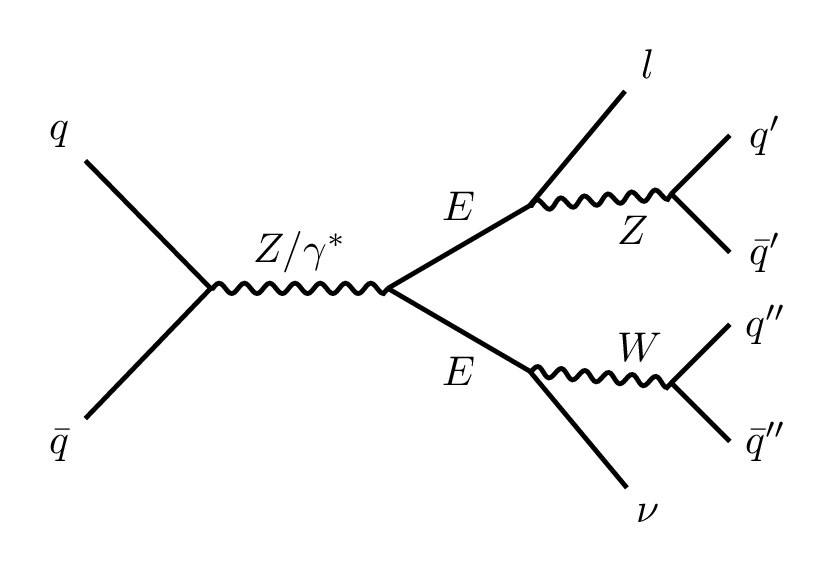
This example only requires the tikz-feynman package. The pdf output can be converted to png as follows.

# Note: Don't use the -alpha remove option if you want transparent png files.
convert -density 300 vll_production.pdf \
-colorspace RGB -quality 90\
-alpha remove -background white\
vll_production.png